Анализ фрактального броуновского движения с помощью непрерывного вейвлет преобразования, с использованием вейвлет мексиканской шляпы

 

Пучков Андрей Александрович,

магистр экономики, докторант Рижского технического университета.

 

Fractal Brownian motion analysis via ‘Mexican hat’ wavelets

 

Andrejs Puchkovs,

Economist, Mg. oec., PhD student of Riga Technical University.

 

This article is dedicated for Fractal Brownian process analysis using Continuous Wavelet Transform (Direct and Inverse). Wavelet Analysis of stochastic processes is very important for financial time series analysis, risk estimation and financial time series forecasting. Wavelet Analysis is very precious for scalability analysis, because of its ability to analyze the signal (process) in scaling and shifting dimensions. In current research, Fractal Brownian motion is analyzed using Direct and Inverse Continuous Wavelet Transform, wavelet coefficients probability density function is estimated, wavelet coefficients lower and upper bounds are calculated using Mexican hat mother wavelet function. At the end estimation results are illustrated.

Nowadays financial market requires a deeper and comprehensive understanding of financial risks. Needs new risk measurement approaches and methods. For many years economists, statisticians, and stock market players have been interested in developing and testing models of stock price behaviour The Hurst exponent, conceptually based on Benoit Mandelbrot Fractal theory and proposed by H. E. Hurst for use in fractal analysis, has been applied to many research fields. This theory was dedicated to extend view of classical Brownian motion using fractal geometry and fractal measure.

 

In Theory the Hurst exponent provides a measure of long-term memory and fractallity of a time series. One of the characteristic indicators of sustainability or persistence of the time series is a constant Hurst - statistic identifying the accumulation and inheritance of the past time series data, the fractal properties of the series. Hurst index (H) can take the values ​​0 ≤ H <1 (from zero to one), and:

1) the values ​​in the range 0 ≤ H <0,5 (from zero to one half) is commonly called pink noise, which has anti-persistent properties;

2) a value of H = 0,5 is called white noise associated with the Brownian motion - the observations are random and uncorrelated, consequently the present value of the time series does not affect the future;

3) the values ​​in the range 0,5 <H <1 indicate the presence of fractal properties of time series, consequently indicate a persistent or trend sustained properties of time series[1].

 

1.                   Fractal Brownian motion

 

Fractal Brownian motion is a continuous-time Gaussian process, which probability distribution function is defined on time t by following equation (1).

                                        (1)

where  F – Fractal Brownian motion probability distribution function; x, u – Fractal Brownian processes, time series; s – Fractal Brownian process standard deviation; t – time; n – time index, integer numbers; H – Hurst exponent.^[2]

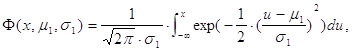
In fact, Fractal Brownian motion probability distribution function can be scripted via normal distribution function by equation (2).

                                            (2)

where Ф – normal distribution function; m₁ – mean of normal distribution function; s₁ – standard deviation of normal distribution function^[3].

Since Fractal Brownian motion probability distribution function can be estimated using normal distribution function, Fractal Brownian motion lower and upper bounds can be found using inverse normal distribution function. See formula (3).

Let,

and                                                                           (3)

then

where Фinv – inverse normal distribution probability distribution function; – probability for lower/upper bounds; X – lower/upper interval bound of Fractal Brownian process at certain probability; x – Fractal Brownian process, time series.

 

2.                   Wavelet analysis

 

Consider  lower/upper interval bound of Fractal Brownian process (at certain probability, and Hurst exponent) is function from t; a signal analysed using direct Continuous Wavelet Transform[4]. Lower/upper interval bound of Fractal Brownian process is scripted by equation (4).

Let,

then 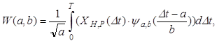                                               (4)

where W – wavelet coefficients; – mother wavelet function; a – scaling parameter; b – shift parameter.[5]

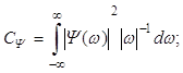
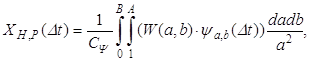
Since Direct Continuous Wavelet Transform is valid, signal synthesis via Inverse Continuous Wavelet Transform can be scripted by formula (5).

                                                                                                       (5)

where C – normalizing coefficient; – Spectral density, Fourier transform of the mother wavelet; A – maximal scales parameter; B – maximal shift parameter.[6]

In accordance with last formula, probability distribution function for wavelet coefficients of Fractal Brownian process can be scripted by equation (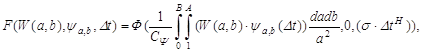6).

                           (6)

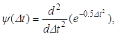
For further analysis, mother wavelet function should be specified. For current research Mexican hat mother wavelet function is chosen. Mexican hat mother wavelet function shifted and scaled can be scripted by formula 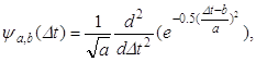(7).

                                                                          (7)

where - mother wavelet function.[7]

In next step, Fractal Brownian process lower/upper interval bound is found (at certain probability measure). Lower/upper interval bound is analysed via Direct Continuous Wavelet Transform using Mexican hat mother wavelet function.

For Fractal Brownian process lower/upper interval bound estimation, following script is used:

 

clc; clear all; close all

output = strcat('J:\Conferences&Publications\Aplimat2013\output\');

 

P = [0.05 0.95];

HH = [0.05 0.25 0.5 0.75 0.95];

 

mu = 0 * ones(size(P));

sigma = 1 * ones(size(P));

tt = 1:256;

 

% Lower Upper Bound Calculation

for Hind = 1:length(HH)

H = HH(Hind);

for t = 1:256

X(:,t,Hind) = norminv(P,mu,sigma.* (t^H));  [8]

end

end

 

i = 0;

a = 1:64;

for Hind = 1:length(HH)

H = HH(Hind);

for Pind = 1:length(P)

Bound = X(Pind,:,Hind);

W(:,:,Pind) = cwt(Bound,a,'mexh'); % Direct CWT                                      

i = i +1; figure('Name',sprintf('%g',i),'Color',[1 1 1])

 

% Create axes

axes1 = axes('FontWeight','light','FontSize',12,...

'FontName','Times New Roman');

 

view([-46.5 34]);

grid('on');

hold('all');

mesh(W(:,:,Pind)) [9]

 

title(['Direct CWT of FBM bounds',sprintf('\n') ,'H =', sprintf('%g',H), ' (P = ',sprintf('%g',P(Pind)),')'],'FontSize',16,'FontName','Times New Roman','FontWeight','demi');

% Create xlabel

xlabel('t (time)');

% Create ylabel

ylabel('scales');

% Create zlabel

zlabel('Wavelet coefficients');

 saveas(gcf,strcat(output,'DCWT_of_FBM_bounds','_H',sprintf('%g',H),'_P',sprintf('%g',P(Pind)),'.jpg'))

end

end

 

Using script provided, following results were found – see next figures.

 

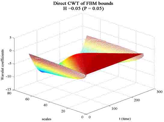
Fig. 1. Wavelet Coefficients of Fractal Brownian process - (H=0,05) lower interval bound at probability measure (P = 0,05).

 

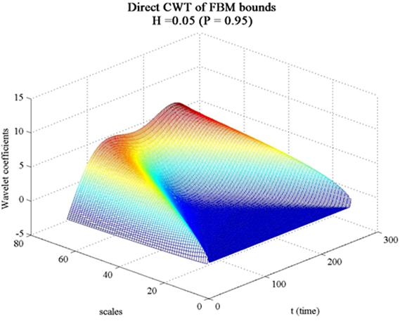
Fig. 2. Wavelet Coefficients of Fractal Brownian process - (H=0,05) upper interval bound at probability (0,95).

 

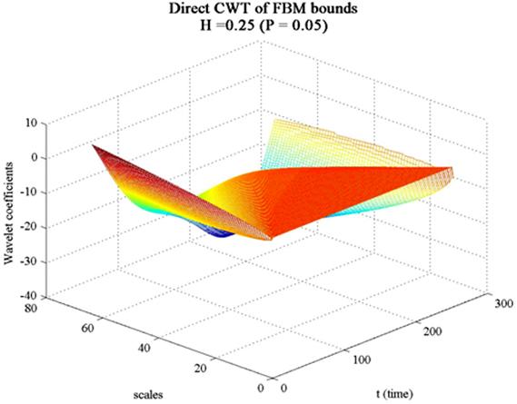
Fig. 3. Wavelet Coefficients of Fractal Brownian process - (H=0,25) lower interval bound at probability (0,05).

 

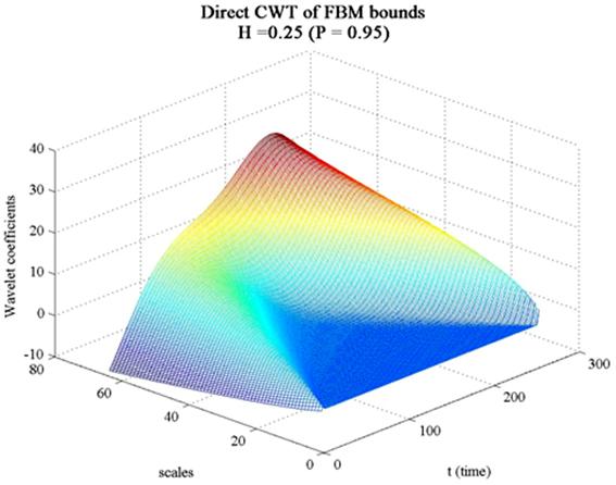
Fig. 4. Wavelet Coefficients of Fractal Brownian process - (H=0,25) upper interval bound at probability (0,95).

 

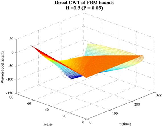
Fig. 5. Wavelet Coefficients of Fractal Brownian process - (H=0,5) lower interval bound at probability (0,05).

 

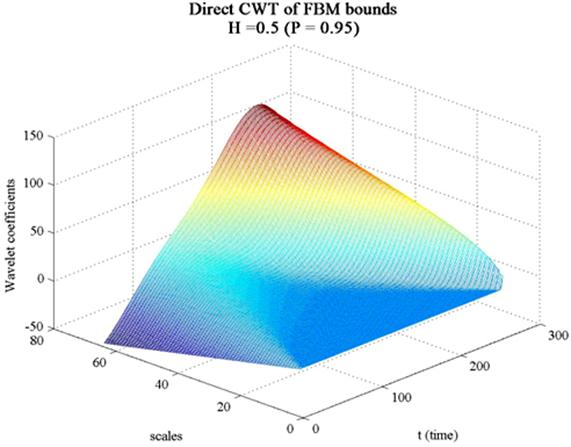
Fig. 6. Wavelet Coefficients of Fractal Brownian process - (H=0,5) lower interval bound at probability (0,95).

 

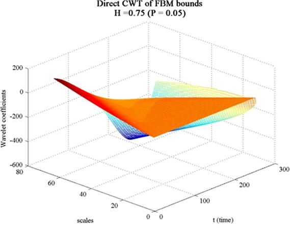
Fig. 7. Wavelet Coefficients of Fractal Brownian process - (H=0,75) lower interval bound at probability (0,05).

 

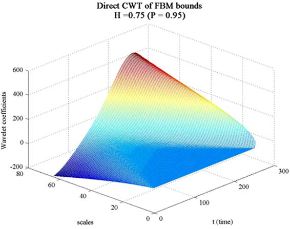
Fig. 8. Wavelet Coefficients of Fractal Brownian process - (H=0,75) upper interval bound at probability (0,95).

 

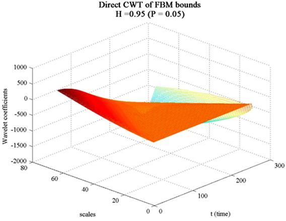
Fig. 9. Wavelet Coefficients of Fractal Brownian process - (H=0,95) lower interval bound at probability (0,05).

 

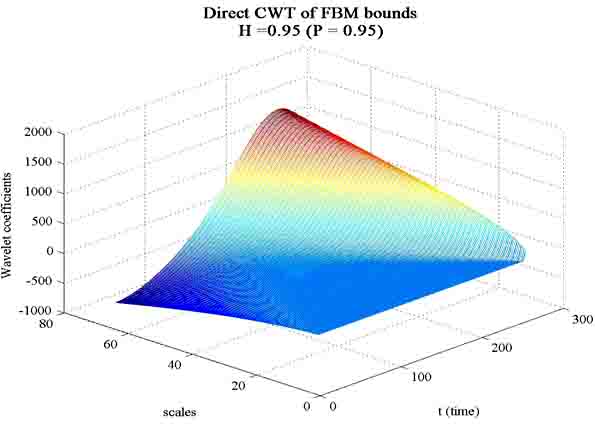
Fig. 10. Wavelet Coefficients of Fractal Brownian process - (H=0,95) /upper interval bound at probability (0,95).

 

Conclusions

 

According to research results, Wavelet coefficients of Fractal Brownian process upper interval bound demonstrate more stability at longest time horizons for higher H (Hurst exponent) values. In this case, Wavelet coefficients form a pyramidal shape with a high centre at large scales and large time horizons.

For lower H (Hurst exponent values) Wavelet coefficients of Fractal Brownian process upper interval bound are quite small. Wavelet coefficients form convex - concave shape with unexpressed peak in the high-scales and mid-time.

Wavelet coefficients for greater Hurst exponent are much divergent from average, while the fractional Brownian process with lower Hurst exponent consistently demonstrates a return to average, so the deviation from average is smaller.

Using Wavelet coefficient probability distribution function Wavelet coefficients of real financial timeseries can be compared to theoretical Wavelet coefficients distribution function of Fractal Brownian Motion at each scaling parameter a. Second implementation of Wavelet coefficients probability distribution function is multifractal process analysis – calculation of scope of fractal measures via thermodynamics partition function and estimation of multifractal spectrums. This branch can be discovered in further research.

 

Bibliography

 

1.                   http://www.johncon.com: Notes on the Fractal Analysis of Various Market Segments in the North American Electronics Industry, [http://www.johncon.com/ndustrix/archive/fractal.pdf], (Accessed 1 January 2013.).

2.                   Кроновер: Фракталы и хаос в динамических системах. Основы. теории. М: Постмаркет, 2000. — 352 с. – 293. стр.

3.                   http://mathworld.wolfram.com: Normal Distribution Function. [http://mathworld.wolfram.com/ NormalDistributionFunction.html] (Accessed 1 January. 2013.).

4.                   http://web.eecs.umich.edu: Mallat's fast wavelet algorithm: recursive computation ofcontinuous-time wavelet coefficients. [http://web.eecs.umich.edu/~aey/eecs551/lectures/mallat.pdf] (Accessed 1 July. 2012.).

5.                   http://en.wikipedia.org: Continuous wavelet transform. [http://en.wikipedia.org/wiki/Continuous_wavelet_transform] (Accessed 1 January. 2013.).

6.                   Яковлев: Введение в вейвлет преобразования. Новосибирск, 2003. – 104 стр.

7.                   http://www.mathworks.se: Norminv - Normal inverse cumulative distribution function. [http://www.mathworks.se/help/stats/norminv.html] (Accessed 1. january 2013).

8.                   http://www.mathworks.se: mesh - Mesh plot. [http://www.mathworks.se/help/matlab/ref/mesh.html] (Accessed 1. january 2013).

 

Поступила в редакцию 15.07.2013 г.