Вычислительные аспекты «Северо-Восточного ветра волатильности»

Вычислительные аспекты «Северо-Восточного ветра волатильности»

Пучков Андрей Александрович,

магистр экономики, докторант Рижского технического университета.

Computational aspects of 'North-East Volatility Wind Effect'

Andrejs Puchkovs,

Economist, Mg. oec., PhD student of Riga Technical University.

This article describes computational aspects of stock index analysis by using wavelet filtering. Such computations are costly from chip-cutting time perspective. Algorithms used for analysis are very important part of research, that's why computational part is described in current paper. Current paper contains also a representation of 'North-East Volatility Wind Effect' in a complex plain, which has not been done before. [6, 7] For exploration of 'North-East Volatility Wind Effect' let's consider basic assumptions.

Analysis of 'North-East Volatility Wind Effect' is based on signal decomposition by using the wavelet filtering. Wavelet filtering is applied by using Direct and Inverse CWT for each scaling parameter. Thus for each scaling parameter the signal component (which is part of the original signal) is obtained. For subsequent research volatility indicator is analyzed by using 20-days time window, which is shifted on the time axis. Volatility analysis is done for each signal component. As a result volatility evolution in time is obtained for each signal component. According to research, a slight increase in volatility in the low-frequency components of the signal leads to significant disturbances in high-frequency components destine entire signal volatility growth.

1. Basic algorithm

Basic algorithm of 'North-East Volatility Wind Effect' analysis is proposed in previous works. [6, 7] Algorithm is shown in the next figure.

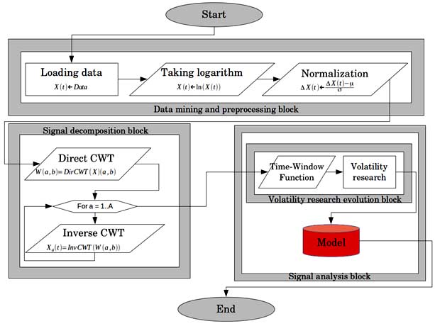
Fig. 1. Algorithm of research.

Research includes three main blocks - Data mining and preprocessing block, Signal decomposition block and Signal analysis block. All blocks are considered in subsequent sections in detail. Research algorithm explanation is made by blocks. All operations and operands in each block are scripted by using Matlab code, which generates figures and/or movies in the output.

The main Matlab code, which runs user functions is shown next:

clear all; clc; close all

%Predefine input and output directories

Stock.Tickets ={'^DJI', '^AEX','^GDAXI','^OMX','^IBEX','^HSI', '^BSESN','^FTSE', '^N225', '^FCHI'};

Stock.Names = {'The Dow Jones Industrial Average',...

'Amsterdam Stock Exchange',...

'DAX30','OMX30','IBEX 35',...

'Hang-Seng Index',...

'S&P BSE SENSEX',...

'FTSE 100',...

'Nikkei 225',...

'CAC 40'};

Stock.N = length(Stock.Tickets);

%Predefine input and output directories

global output plotedir

output = '/Code/';

plotedir = '/Plots/';

savecode = strcat(output,'metadata.mat'); save (savecode);

for yy = 1:Stock.N

output = '/Code/';

plotedir = '/Plots/';

savecode = strcat(output,'metadata.mat');

load (savecode)

%Recalculate

recalc = [0 0 0 0 0]; %<- recalculate selected functions

%Data mining and preprocessing

[ind,tickname, tick,stdate,endate] = deal(yy,Stock.Names{yy}, Stock.Tickets{yy},datenum(2004,1,1),datenum(2014,1,1));

[Signal.X, Signal.dX, Signal.t, Signal.T] = lo_pro(recalc(1),ind, tickname, tick, stdate, endate, true);

clear stdate endate

%Signal decomposition

[Wavelet.W, Decomp.X_ab, Decomp.X_cap] = wave_an(recalc(2), ind, tickname, tick, Signal.X, true);

% Volatility analysis

[Volatility.Vol, Volatility.a, Volatility.da, Volatility.db] = var_an(recalc(3), ind, tickname, tick, Decomp.X_ab, Signal.X, true);

% Volatility evolution

[Volevol] = var_ev_nomovie(recalc(4), ind,tick,tickname, Volatility.Vol, Volatility.a, true);

clear all; close all;

end

This code is used to download historical price data for specified stock indexes, preprocessed the data, decomposed signal in parts and make volatility analysis of specified parts (or components). Further this code runs volatility evolution analysis to describe interdependences between volatility layers. At the end code makes volatility evolution representation in complex plain. All this parts of algorithm are executed, by running Matlab user-defined functions, which are saved in the same directory.

2. Data Mining and Preprocessing Block

This block intend for financial data mining and preprocessing. The block is placed before Signal decomposition and analysis blocks. Data mining and preprocessing block has three main elements: Data loading operation, Taking logarithm operand and Normalization operand. ’Loading data’ operation is completed in early beginning by using automatic financial time series data download from ’finance.yahoo.com’ source.

Those parts of algorithm are realized by using lo_pro.m function:

function [X, dX,t,T] = lo_pro(recalc,ind,tickname, tick,stdate,endate,showplot)

%Input:

% recalc - do calculations if true;

% ind - [tickets{ind} = ticket];

% tick - stock index ticket;

% sdate, endate - startdate nd enddate;

% showplot - if true, plotting is provided;

%Output:

% X - the signal;

% dX - growth of the signal;

% t - time space

% T - length of signal

%_________________________________________________________________________%

global output plotedir

lofname = strcat(output,'lprocess',num2str(ind),'.mat');

if(exist(lofname,'file') == 2)

load (lofname)

if ((exist('X','var') == 1) &&...

(exist('dX','var') == 1) &&...

(exist('t','var') == 1) &&...

(exist('T','var') == 1))

varex = true; % - variables already exist (and file too)

else

varex = false;

end

else

varex = false;

end

if ((recalc == true) || (varex == false))

% Loading data

Data = get_yahoo_stockdata2(tick,stdate,endate,'d',true);

XD = Data.Close;

XD = log(XD);

% Signal preprocessing

wn = diff(XD);

% Normalization

dX = (wn - mean(wn))./std(wn);

%Time

T = length(dX); t = 1:T;

%Create signal

X = cumsum(dX); %Correction needed: XD(1) + X;

save(lofname, 'X', 'dX', 't', 'T','-append')

disp(strcat('load_process variables for ...', tick,'... are REcalculated!'))

%Plotting

draw_plot(showplot,recalc,plotedir,ind, tickname, tick, t, X, dX);

else

disp(strcat('load_process variables for ...', tick,'... are already calculated'))

%Plotting

draw_plot(showplot,recalc,plotedir,ind, tickname, tick, t, X, dX); %#ok

return

end

%Plotting function

function draw_plot(showplot,recalc,plotedir,ind, tickname, tick, t, X, dX)

if(showplot)

subdir = 'Signal/';

drawjpg = strcat(plotedir,subdir,num2str(ind),'_','Signal',num2str(tick),'.jpg');

if (recalc) || ~(exist(drawjpg,'file') == 2)

figure(1)

subplot(2,1,1), plot(t,X)

title(strcat('Analysed Signal - ', num2str(tickname)),'Interpreter','none','FontSize',15);

xlabel('Time, t','Interpreter','none','FontSize',12);

ylabel('INDEX, X','Interpreter','none','FontSize',12);

axis( [0 t(end) min(X) max(X)] )

subplot(2,1,2), plot(t,dX)

title(strcat('Signal Additions - ', num2str(tickname)),'Interpreter','none','FontSize',15);

xlabel('Time, t','Interpreter','none','FontSize',12);

ylabel('INDEX ADDITIONS, dX','Interpreter','none','FontSize',12);

axis( [0 t(end) min(dX) max(dX)] )

saveas(gcf,drawjpg)

disp(strcat('File...',drawjpg,'... is provided'))

close all;

else

disp(strcat('File...',drawjpg,'... already exist'));

end

This function imports and process financial data (in case it was not done before and user have not defined option to recalculate). By analogy code provides pictures of processed signal and signal signal additions to specified directory, if user have defined such option by using argument showplot.

3. Signal decomposition block

Signal decomposition block is placed between Data mining and preprocessing block and Signal analysis block. The block consist of two parts: Direct Continuous Wavelet Transform (Direct CWT) and Inverse Continuous Wavelet Transform (Inverse CWT) operands. [2, 3] Since analyzed signal is decomposed in parts, Direct CWT and Inverse CWT operands are working in loop, providing decomposed parts of analyzed signal for each scaling parameter. [9] In the output Signal decomposition block provides decomposed parts of the signal for each scaling parameter, in fact, these are components of (original) analyzed signal, which are analyzed separately in the Signal analysis block.

This algorithm are realized by using wave_an.m function:

function [W, X_ab, Xcap] = wave_an(recalc, ind, tickname, tick, X, showplot)

%Input:

% recalc - do calculations if true;

% X - the signal;

% ind - [tickets{ind} = ticket];

% tick - stock index ticket;

%Output:

% W - Wavelet image

% X_ab - decomposed signal;

% Xcap - reconstructed signal;

% log_Xab - logged decomposed signal;

%_________________________________________________________________________%

global output plotedir

lofname = strcat(output,'lprocess',num2str(ind),'.mat');

if (exist(lofname,'file') == 2)

load (lofname)

if ((exist('W','var') == 1) &&...

(exist('X_ab','var') == 1) &&...

(exist('Xcap','var') == 1) &&...

(exist('log_Xab','var') == 1))

varex = true; % - variables already exist (and file too)

else

varex = false;

end

else

varex = false;

end

if ((recalc == true) || (varex == false))

% Wavelet analysis

% Define parameters before analysis

dt = 1;

maxsca = floor(T); s0 = 2*dt; ds = 2*dt;

wname = 'morl';

scales = s0:ds:maxsca; A = length(scales);

SIG = {X,dt};

WAV = {wname,[]};

% Compute the CWT using cwtft with linear scales

W = cwtft(SIG,'scales',scales,'wavelet',WAV);

Wx = W; Wx.cfs = zeros(2,T);

X_ab = zeros(length(scales),T);

for a = 1: A

if (a < A)

Wx.scales = scales(a:a+1);

else

Wx.scales = [A A+ds];

end

Wx.cfs(1,:) = W.cfs(a,:);

%Inverse CWT:

X_ab(a,:) = icwtlin(Wx);

mu = mean(X_ab(a,:));

X_ab(a,:) = (X_ab(a,:) - mu);

end

% Adding constant for perfect reconstruction

Xcap = sum(X_ab)';

C = mean(X-Xcap);

C = C/A;

X_ab = X_ab + C;

Xcap = sum(X_ab)';

x_pl = (X_ab>0); x_mi = (X_ab<=0);

X_abs = abs(log(X_ab));

log_Xab = X_abs.*x_pl - X_abs.*x_mi;

%Saving output

save(lofname, 'W', 'X_ab', 'Xcap', 'log_Xab','-append')

draw_plot(showplot,recalc,plotedir,ind, tickname, tick, log_Xab);

disp(strcat('Signal decomposition for ...', tick,'... ISprovided!'))

else

draw_plot(showplot,recalc,plotedir,ind, tickname, tick, log_Xab); %#ok

disp(strcat('Signal decomposition for ...', tick,'... is already provided'))

return

end

function draw_plot(showplot,recalc,plotedir,ind, tickname, tick, log_Xab)

if(showplot)

subdir2 = 'Decomp/'; %subdir1 = 'Wavelet/';

drawjpg = strcat(plotedir,subdir2,num2str(ind),'_','Decomp',num2str(tick),'.jpg');

if (recalc) || ~(exist(drawjpg,'file') == 2)

[A,B] = size(log_Xab);

figure(1);

subplot(2,2,1),mesh(log_Xab)

axis ([0 B 0 A]);

view(-45, 60);

title(strcat('Decomposed Signal Parts - ', num2str(tickname), ' view1'),'Interpreter','none','FontSize',15);

xlabel('Shift parameter, b','Interpreter','none','FontSize',12);

ylabel('Scaling parameter, a','Interpreter','none','FontSize',12);

subplot(2,2,2),mesh(log_Xab)

axis ([0 B 0 A]);

view(0, 90);

title(strcat('Decomposed Signal Parts - ', num2str(tickname), ' view2'),'Interpreter','none','FontSize',15);

xlabel('Shift parameter, b','Interpreter','none','FontSize',12);

ylabel('Scaling parameter, a','Interpreter','none','FontSize',12);

subplot(2,2,4),mesh(log_Xab)

axis ([0 B 0 A]);

view(45, -60);

title(strcat('Decomposed Signal Parts - ', num2str(tickname), ' view3'),'Interpreter','none','FontSize',15);

xlabel('Shift parameter, b','Interpreter','none','FontSize',12);

ylabel('Scaling parameter, a','Interpreter','none','FontSize',12);

subplot(2,2,3),mesh(log_Xab)

axis ([0 B 0 A]);

view(180, -90);

title(strcat('Decomposed Signal Parts - ', num2str(tickname), ' view4'),'Interpreter','none','FontSize',15);

xlabel('Shift parameter, b','Interpreter','none','FontSize',12);

ylabel('Scaling parameter, a','Interpreter','none','FontSize',12);

saveas(gcf,drawjpg)

disp(strcat('File...',drawjpg,'... is provided'));

close all;

else

disp(strcat('File...',drawjpg,'... already exist'));

end

This function decompose financial data in parts by using Direct an Inverse Continuous Wavelet Transform. Since this operations are very costly from chip-cutting time perspective, in case there is no option for recalculation, code tries to find saved or already calculated data. The code also provides pictures of decomposed signal parts to specified directory, if user have defined such option by using argument showplot.

4. Signal analysis block (volatility analysis)

This block brings light on volatility evolution research. The block is placed after Signal decomposition block and it works with decomposed parts of analyzed signal. Signal decomposition, made in previous step, has divided original signal in components by using wavelet filtration. The purpose of current research is volatility analysis and volatility evolution analysis.

Volatility research is realized by using var_an.m function:

function [Vol, Vol_a, Vol_da, Vol_db] = var_an(recalc, ind, tickname, tick,X_ab,X,showplot)

%Input:

% recalc - do calculations if true;

% ind - [tickets{ind} = ticket];

% tick - stock index ticket;

% X_ab - decomposed signal;

% X - the signal;

%Output:

% Vol - Overall signal Volatility

% Vol_a - Volatility of decomposed parts of the signal

% Vol_da - Volatility indicator (of decomposed parts)

% Vol_db - Volatility indicator (of decomposed parts)

%_________________________________________________________________________%

global output plotedir

lofname = strcat(output,'lprocess',num2str(ind),'.mat');

if (exist(lofname,'file') == 2)

load (lofname)

if ((exist('Vol_a','var') == 1)&&...

(exist('Vol_da','var') == 1)&&...

(exist('Vol_db','var') == 1)&&...

(exist('Vol','var') == 1))

varex = true; % - variables already exist (and file too)

else

varex = false;

end

else

varex = false;

end

if ((recalc == true) || (varex == false))

%Predefine papameters

daX_ab = log(diff(X_ab));

dbX_ab = log(diff(X_ab'))';

[A, B] = size(daX_ab);

win = 20; del = 5;

%Volatility analysis

for a = 0:A

st = 1;

en = st + win;

bmod = 1;

if (a == 0)

while (en < B)

st = st + del;

en = st + win;

bmod = bmod +1;

end

Vol_a = zeros(A,bmod-1); %define margins

Vol_da = Vol_a; Vol_db = Vol_a;

Vol = zeros(bmod-1,1);

else

while (en < B)

if(a ==1),

Vol(bmod) = var(X(st:en));

end

Win1= X_ab(a,st:en); %define window

Vol_a(a,bmod) = log(var(Win1)); %variance

Win2 = daX_ab(a,st:en); %define window

Vol_da(a,bmod) = log(var(Win2)); %variance indicator

Win3 = dbX_ab(a,st:en); %define window

Vol_db(a,bmod) = log(var(Win3)); %variance indicator

st = st + del;

en = st + win;

bmod = bmod +1;

end

save(lofname, 'Vol_a', 'Vol_da', 'Vol_db','Vol','-append')

draw_plot(showplot,recalc,plotedir,ind, tickname, tick, Vol_a, Vol_da, Vol_db)

disp(strcat('Volatility analysis for ...', tick,'... ISprovided!'))

else

draw_plot(showplot,recalc,plotedir,ind, tickname, tick, Vol_a, Vol_da, Vol_db) %#ok

disp(strcat('Volatility analysis for ...', tick,'... is already provided'))

return

end

function draw_plot(showplot,recalc,plotedir,ind, tickname, tick, Vol_a, Vol_da, Vol_db)

if(showplot)

subdir = 'Volatility/';

drawjpg = strcat(plotedir,subdir,num2str(ind),'_','Volatility',num2str(tick),'.jpg');

if (recalc) || ~(exist(drawjpg,'file') == 2)

[A,B] = size(Vol_a);

figure(1);

subplot(2,2,1),mesh(Vol_a)

axis ([0 B 0 A]);

view(0, 90);

title(strcat('Volatility layers - ', num2str(tickname), ' view1'),'Interpreter','none','FontSize',15);

xlabel('Shift parameter, b','Interpreter','none','FontSize',12);

ylabel('Scaling parameter, a','Interpreter','none','FontSize',12);

subplot(2,2,2),mesh(Vol_a)

axis ([0 B 0 A]);

view(-45, 60);

title(strcat('Volatility layers - ', num2str(tickname), ' view2'),'Interpreter','none','FontSize',15);

xlabel('Shift parameter, b','Interpreter','none','FontSize',12);

ylabel('Scaling parameter, a','Interpreter','none','FontSize',12);

subplot(2,2,4),mesh(Vol_da)

axis ([0 B 0 A]);

view(0, 90);

title(strcat('Volatility differential (by scaling a) - ', num2str(tickname)),'Interpreter','none','FontSize',15);

xlabel('Shift parameter, b','Interpreter','none','FontSize',12);

ylabel('Scaling parameter, a','Interpreter','none','FontSize',12);

subplot(2,2,3),mesh(Vol_db)

axis ([0 B 0 A]);

view(0, 90);

title(strcat('Volatility differential (by shift b) - ', num2str(tickname)),'Interpreter','none','FontSize',15);

xlabel('Shift parameter, b','Interpreter','none','FontSize',12);

ylabel('Scaling parameter, a','Interpreter','none','FontSize',12);

saveas(gcf,drawjpg)

disp(strcat('File...',drawjpg,'... is provided'));

close all;

else

disp(strcat('File...',drawjpg,'... already exist'));

end

This function provides 20-days volatility indicator of financial data for each part of the signal. The code provides pictures of volatility research and derivatives. With them it is possible to trace volatility evolution in time for each volatility layer.

Volatility evolution and complicated interdependencies between volatility layers can be discovered by using user defined Matlab function var_ev_nomovie.m.

function [Volevol] = var_ev_nomovie(recalc, ind,tick,tickname, Vol, Vol_a, movie)

%Input:

% recalc - do calculations if true;

% ind - [tickets{ind} = ticket];

% tick - stock index ticket;

% Vol_a - Volatility of decomposed parts of the signal;

%Output:

% Volevol - object, containing:

% Volevol.volfile - paths and filenames of .mat files containing: % variables;

% Volevol.FileN - number of .mat files containing variables

% Volevol.Vars - variables (to be read);

% Evol - volatility changes;

% Bind - indexed B values (shift or time values);

% matrix

% Volevol.VarN - number of variables;

%_________________________________________________________________________%

global output plotedir

lofname = strcat(output,'lprocess',num2str(ind),'.mat');

if (exist(lofname,'file') == 2)

load (lofname)

if ((exist('Volevol','var') == 1))

varex = true; % - variables already exist (and file too)

else

varex = false;

end

else

varex = false;

end

if ((recalc == true) || (varex == false))

% Volatility evolution analysis

[A, B] = size(Vol_a);

Packsize = 50;

Evol = zeros(A, A, Packsize);

Bind = zeros(Packsize,1);

Volevol.Vars{1} = 'Evol';

Volevol.Vars{2} = 'Bind';

Volevol.VarN = 2;

ii = 0; j = 0; blast = B-1;

for b = 1:blast

ii = ii+1;

Lay1 = Vol_a(:, b);

Lay2 = Vol_a(:, b+1);

Laydim1 = repmat(Lay1, 1, A);

Laydim2 = repmat(Lay2', A, 1);

Evol(:,:,ii) = Laydim2-Laydim1;

Bind(ii) = b;

if (ii >= Packsize) || (b == B-1)

j = j +1;

Volevol.volfile{j} = strcat(output,'Volatility/','Volwind',num2str(ind),'-',num2str(j), '.mat');

save (Volevol.volfile{j}, Volevol.Vars{1},Volevol.Vars{2});

Evol = zeros(A, A, Packsize);

Bind = zeros(Packsize,1);

ii = 0;

disp(strcat('j = ',num2str(j),'; Time = ', num2str(CT)));

end

Volevol.FileN = j;

save(lofname, 'Volevol','-append')

Volevol.R = extract_vol(movie,recalc, plotedir,ind,tick,tickname,Volevol,Vol,Vol_a);

disp(strcat('Volatility evolution analysis for ...', tick,'... ISprovided!'))

else

Volevol.R = extract_vol(movie,recalc, plotedir,ind,tick,tickname,Volevol,Vol,Vol_a); %#ok

disp(strcat('Volatility evolution analysis for ...', tick,'... is already provided'))

return

end

function [R] = extract_vol(movie,recalc, ~,~,~,~,Volevol,~,Vol_a)

if(movie)

if (recalc)

[~, B] = size(Vol_a); B = B-1;

bind = 0;

for j = 1:Volevol.FileN

f_n = Volevol.volfile{j};

load(f_n,'Evol')

[~, ~, zn] = size(Evol); %#ok

z = 1;

while (z <= zn) && (bind<B)

Del_Vol = Evol(:,:,z);

[~,~,~,Hr,rv] = sc2_rad(Del_Vol,'','calcradar');

bind = bind+1;

R.Hr(:,z) = Hr;

R.rv(:,z) = rv;

disp(num2str(z))

z = z+1;

end

clear Evol

end

else

end

close all;

end

This code is very expensive from chip-cutting time perspective, on the other hand it brings a very detailed picture of volatility evolution and interdependencies between volatility layers. Actually this code provides only object, which contains information of stored data, the data is very big ~ 110 GB of data for each stock index.

This function is running sc2_rad.m function, which is user defined function, which is providing volatility evolution picture in complex plain, which has not been discovered yet.

5. Volatility analysis in a complex plain

Transmission of volatility between layers which is calculated in previous function by using argument Del_Vol can be represented in a complex plain, for such transformation coordinates x,y of Del_Vol matrix are rewritten in following form. [1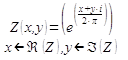1].

(1)

This transformation and fuhrer research is realized in following Matlab code:

function [Xr,Yr,Zr,Hr,rv] = sc2_rad(Matrx,addplot,radarvalue)

[x,y,z] = find(Matrx);

Z_Num = x + y*1i;

appi = (pi);

Z_exp = exp(Z_Num/(2*appi));

x = real(Z_exp);

y = imag(Z_exp);

rxy = log(sqrt(x.^2 + y.^2))./(sqrt(x.^2 + y.^2));

x = x.*rxy;

y = y.*rxy;

F = scatteredInterpolant(x,y,z,'natural');

%disp('calculated 001');

N = 1000;

xmin = min(x); xmax = max(x); xvec = linspace(xmin,xmax,N);

ymin = min(y); ymax = max(y); yvec = linspace(ymin,ymax,N);

[X,Y] = meshgrid(xvec,yvec);

%disp('calculated 0015')

qz = F(X, Y);

%disp('calculated 002');

[xc,yc] = meshgrid(linspace(-1,1,N));

cir = (xc.^2 + yc.^2 <=1);

qz = cir.*qz;

qz = abs(qz);

%disp('calculated 003');

Hr = zeros(N,1);

switch radarvalue

case 'calcradar'

dr = 0.01;

r0 = 0;

i = 1;

rv(i) = r0+dr;

while r0+dr <1

boolcir = (sqrt(xc.^2 + yc.^2) >r0) & (sqrt(xc.^2 + yc.^2) <= r0+dr);

Obj = qz.*boolcir;

Hr(i) = mean(mean(Obj > 0));

rv(i) = r0+dr;

r0 = r0 + dr;

i = i + 1;

end

otherwise

end

Xr = X;

Yr = Y;

Zr = qz;

switch addplot

case 'radarplot'

figure;

mesh(X, Y, qz);

axis tight

figure

plot(Hr)

otherwise

end

This code provides a radar picture of volatility evolution and a much clearer picture of transmition of volatility between volatility layers. In the output code provides volatility indicator which is normalized to radius. Representation of volatility transmission in radial form brings out better understanding of volatility nature nad brings light on 'North-Ease Volatility Wind Effect'.

Bibliography

1. Кроновер. Фракталы и хаос в динамических системах. Основы. теории. М: Постмаркет, 2000. — 352 с. – 293. стр.

2. Смоленцев. Основы теории вейвлетов в MATLAB. М: ДМК Пресс, 2003. - 304. стр.

3. Яковлев. Введение в вейвлет преобразования. Новосибирск, 2003. – 104 стр.

4. Mathworks.com. Continuous 1-D wavelet transform.[http://www.mathworks.se/help/wavelet/ref/cwt.html] (Accessed 1 January. 2014).

5. Mathworks.com. Continuous wavelet transform using FFT algorithm.[http://www.mathworks.se/help/wavelet/ref/cwtft.html] (Accessed 1 January. 2014).

6. Mathworks.com. Inverse CWT.[http://www.mathworks.se/help/wavelet/ref/icwtft.html] (Accessed 1 January. 2014).

7. PUCKOVS, A., MATVEJEVS, A.: Equity Indexes Analysis and Synthesis by using Wavelet Transforms. CFE 2013 7-th International Conference on Computational and Financial Econometrics, London: Birkbeck University of London, 2013, ISBN 978-84-937822-3-8, p. 98.

8. PUCKOVS, A., MATVEJEVS, A.:’North-East Volatility Wind’ Effect. No: 13th Conference on Applied Mathematics (APLIMAT 2014): Book of Abstracts: 13th Conference on Applied Mathematics (APLIMAT 2014), Slovakia, Bratislava, 4.-6. Feb., 2014. Bratislava: 2014, 67.-67.pp. ISBN 9788022741392.

9. TREFETHEN, L. N. Spectral Methods in MATLAB. Comlab, 2007, 160 s.

10. Youtube.com. Advanced Digital Signal Processing-Wavelets and multirate by Prof.v.M.Gadre,Department of Electrical Engineering, [http://www.youtube.com/watch?v=RBZQDBNdzWk&list=PLarWa9wEKs_H3Go20IYoDR26t6XnX6tZj] (Accessed 1 January. 2014).

11. www.youtube.com Complex Number. [http://www.youtube.com/watch?v=b3adw5igSzI] (Accessed 1 January. 2014.).

12. www.youtube.com Complex Number Theory. [http://www.youtube.com/watch?v=b3adw5igSzI] (Accessed 1 January. 2014.).

13. Youtube.com. Lecture Series on Digital Signal Processing by Prof.T.K.Basu, Department of Electrical Engineering, IIT Kharagpur. [http://www.youtube.com/watch?v=V-kLaH4139o&list=PLBC201E07F0818B5A] (Accessed 1 January. 2014).

14. Youtube.com. Lecture Series on Digital Voice and Picture Communication by Prof.S. Sengupta, Department of Electronics and Electrical Communication. [http://www.youtube.com/watch?v=kp2zPGpKd74] (Accessed 1 January. 2014).

Поступила в редакцию 15.05.2014 г.