Автоматизированная система управления плотностью движения магистрали

 

Абдул Салаам Авад Кадхим Ал Хазражи,

университет Гармиан, Ирак.

 

Automated highway System with Traffic Density Control

 

Dr. Abdul Salam. A. Al-Khazraji,

Fac. of Education – University of Garmian, Kurdistan Region – Iraq.

 

On the macroscopic level a roadway controller calculates the desired speed Commands to be followed by vehicles in each section of the freeway lanes in order to achieve desired traffic density distribution that lead to optimum traffic flow conditions.

In this paper we deign, analyze & simulate a roadway Controller for an automated highway that achieves desired traffic densities along the lane.

A macroscopic traffic flow model that is modified for (AHS) operation is used for control design & analysis.

We show that the proposed roadway controlled guarantees exponential convergence of the traffic density at each section to the desired density. Simulation results are used to illustrate the effectiveness of the proposed controller & the significant benefits (AHS) may bring to traffic flow.

Keywords: Macroscopic traffic flow: roadway controller: traffic flow density control: automated highway systems.

 

1.                   Traffic Flow Model

The analogy between traffic flow and fluid flow formed the basis for the first traffic flow model.

 

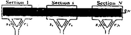
Fig. 1.

 

Consider a single freeway lane, which is subdivided into N sections with lengths , as shown in Fig. 1.

The space- and time-discretized traffic flow model for a segment of the lane involves the following variables:

 density in section i at time nT (in vehicles per kilometer per lane), where

 space mean speed of vehicles in section I, at time nT (

 traffic volume leaving section i, entering section  at time nT (in vehicles per hour);

 on-ramp traffic volume for section i (in vehicles per hour);

 off-ramp traffic volume for section i (in vehicles per hour):

 length of ith section (in km);

T time-discretization step size (in h).

The modified freeway traffic flow model given in Karaaslan et al. (1990) is in the following form:

 {

Where

,

Here  and  are positive constants with , and k_jam is the maximum possible density. The variable  in (3) represents the density-dependent equilibrium speed. In a manual operating environment with homogeneous traffic conditions. this re­lationship has been characterized in Papageor. giou (1989) and Papageorgiou ei al (1990a, b) as

where  and  arc real-valued parameters, and V_t, is the free speed, which can be estimated from traffic data.

The term  in (3) under manual operation depends on the downstream density, and can be expressed as

where the positive constant K is introduced to prevent abnormal growth of the velocity for section i when its density is very low,

Typical parameter values associated with the above model are given in Table 1.

 

2.                   Boundary conditions

We assume that the traffic flow rate entering section 1 during the time period nT and  is  and the mean speed of the traffic entering section 1 is equal to the mean speed of section  In addition, we also assume that the mean speed and traffic density of the traffic exiting section N + 1 are equal to those of section  Hence the boundary conditions for the entrance and exit can be summarized as follows:

The physical meaning of each term of (3) that influences the mean speed of a section can be interpreted as follows (Papageorgiou, 1983, Karaaslan et aL, 1990).

Thc second term,  is the relaxation term, which accounts for the evolution of the mean speed  towards its density dependent equilibrium :speed  with a time constant  The dependence of  on the density is influenced by the environment in which the traffic flow is operating For manual operation_, this relationship is governed by (4), as reported in Papageorgiou (1989) and Papageorgiou et al (1990 a.b). For an AHS operating under homogeneous heavy traffic conditions, the adopted safety policy for vehicles defines this relationship. For instance, if the desired safety distance between two vehicles Sa is made to depend on the equilibrium velocity

then the density equilibrium speed relationship can he characterized by      

Where  is the inverse function of  satisfies the equation  If the constant-time headway policy is adopted for selecting the inter vehicle spacing then.

where h and c are constants. It follows that

The third term

in (3) is the convection term. It represents the influence of the incoming traffic on the mean speed evolution in segment i.

The last term, - in (3) is the anticipation term. For manual driving, human drivers in general increase or decrease vehicle speed, depending on the traffic density downstream. In other words, for manual driving, the anticipation term reflects the effect of downstream traffic density on the mean speed evolution in section i at sampling time nT. For instance, if the density downstream is lower. this term reflects the tendency of human drivers to increase vehicle speed. More specifically, the anticipation term represents the microscopic traffic dynamics that describes the interaction between vehicles or vehicles' response to the down stream's traffic conditions: For AHS, the anticipation term no longer represents the tendency of the human driver's response to the down stream's traffic conditions. Instead, It represents the microscopic traffic dynamics governed by the AHS control system.

 

Table 1.

Parameters associated with the traffic model.

 

The complete traffic model under manual operation is described by (1)-(4), with w_(n) defined in (5)‑

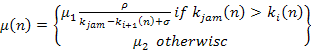
The dynamics of traffic flow in AHS are still described by (1) -(3), but the adopted safety policy that defines the equilibrium speed-density relationship (10) replaces (4). Furthermore, the designed control law u(n) replaces the last term in (3). The complete behavior of traffic flow in AIIS is governed by the following equations:

 

Here are positive constants, with is the inverse function of the adopted safety policy .

 

3.                   Problem Statement

Traffic congestion in urban freeways is caused by ad hoc velocities and headway's that humans choose when they operate their vehicles. Therefore any strategy that hopes to reduce congestion needs to remove this human subjective element and replace it with a method that directly controls the density and speed of vehicles by

prescribing speed commands to vehicles in each section of the highway.

Assume that the roadway has the capability of measuring mean speeds and traffic densities at each section of a lane. The goal of traffic management is to assess the state of the traffic and provide appropriate speed commands to the vehicles at various sections of the lane in order to maintain a desired traffic density profile that under the current traffic conditions corresponds to some optimum traffic flow situation. A roadway controller can he designed to perform this task. The speed commands should be generated so that the desired traffic flow rate can be achieved and the density distribution along the lane leads to a homogeneous traffic flow.

Consider a lane subdivided into N sections with lengths L,, i = 1, ... N. as shown in Fig. 1. The traffic now rate entering section 1 at sampling time nT is q_o(n) vehicles per hour. The desired traffic density for section f of a single lane is assumed to be k_d(n).

Our objective is to choose a proper value of u,(n) for section r such that the traffic density of section i converges to the desired traffic density kw(n) exponentially fast, i.e k₁(n)+k_d (n) as .

 

4.                   A Roadway Traffic Density Controller

In this section, we propose a microscope roadway traffic density controller for AHS. Our design uses integrator back stepping to realize the control law needed to track a desired density profile The following general lemma Is used ,n

the design and analysis of the proposed roadway controller.

Lemma 1. Consider the following discrete-lime system:

where c is a constant and  exponentially implies z(n)-.0 exponentially.

Proof. This is trivial and is omitted.

The main idea of the controller design is to apply back stepping and use Lemma 1 over and over again. That is, we treat v₁(n) as a free variable in (12) to control the density k₁(n + 1) at the next time point. Then the desired control action of u₁(n) is achieved by designing the control input v₁(n) utilizing (13).

The control design consists of three steps.

Step 1. We begin out design by defining the tracking error for section f as

Then, with (12), it follows that

Where

From Lemma 1_, we have  and  as . The goal of the next step is to choose the control input  that guarantees  as

Step 2. From the definition of  and (II), we have

To simplify the notation, we define

We have from (12) and (15) that

Therefore. the quantities   are available at sampling time nT. To stress this fact, we define

Substituting out definitions (18)-(21) into (17). we obtain the compact form

Then, with (22), it follows that

We now consider the dynamics of this equation for the entrance . exit  and intermediate sections  of the freeway lane. Let us first define

Than, using (13) and (25) , we have

Case  for intermediate freeway sections. Using (24) and (26). we have

 …..…… (27)

Where

 …… (28)

Therefore is we choose the control signal  to satisfy

And choose  application of Lemma 1 to (27), we have

Case  entrance. Using the boundary condition (7) in (24). we have

Substituting for a₁(n) and b₁(n) from (22). (18) and (19) in this equation and using the boundary condition (6), we have

     ...

Where

Therefore if we choose the control u,(n) to satisfy

then, by applying Lemma 1 to (31), we have

Case  for freeway exit. Using the boundary condition (9) in (24). we have

 

Substituting for bn(n) and _cn(n) from (22), and (19) and (20) in this equation and using the boundary condition (8), we have

Where

Therefore is we choose the control to satisfy

then, by applying Lemma 1 to (35), we have

Step 3. To obtain the control law u,(n), i = 1, 2, . N from (29), (33) and (37), we need to solve the algebraic equation

Where

and

We define two constants , and where

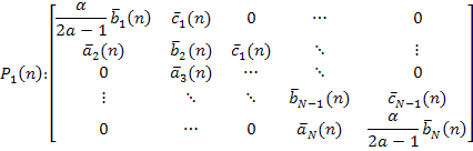
Substituting (41) and (42) into the tridiagonal matrix equation (38) yields

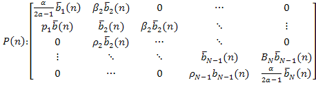
The uniqueness of the solution of (43) depends on the non-singularity of P(n). which in turn can be guaranteed if

for some constant.

To ensure satisfaction of this condition, we make the following assumption for each section of the freeway lane at any sampling time.

Assumption 2. (Traffic flow controllability). There exists a small positive constant such that , n,

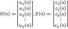
Theorem 3 Assume that the traffic flow controllability stated in Assumption S is satisfied for each section at any sampling time. Leta be a positive constant defined as in Table I. Let P(n), U(n) and E(n) be as defined in (44) in (40). Then there exist control inputs u,(n) satisfying

that drive the traffic density k,(n) for section i,i = 1, 2, .... N to the desired traffic density k₄(n) exponentially fast.

Proof. We showed in Step 3 that the desired control taw must satisfy the matrix equation (45). This provides the solution of the algebraic equations (29), (33) and (37) in Step 2. Application of Lemma 1 along with this solution to (27). (31) and (35) yields

 as  The use of the same lemma with (16) ensures that   Hence  we have  exponentially.

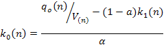
Theorem 3 provides the control strategy needed for tracking a desired density profile. According to this theorem and (13), if u,(n) is chosen as (45), the average velocity in each section i of the lane at sampling time (n + 1)T will be

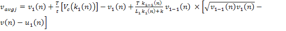
and the traffic density at section t converges to the desired traf^fic density k₄ exponentially.

Consider a long segment of freeway, which is divided into 12 sections. The length of each section is 500 at. The initial traffic volume entering section 1 is assumed to be 1500 vehicles per hour. The initial density and mean speed of each section are as shown in Table 2.

Four cases are considered. In the first, shown in Figs 2 and 3, no feedback from the roadway is applied, and therefore u,(n) is replaced with the corresponding term in (3). From these figures, we see the propagation of congestion upstream due to the initial traffic congestion in sections 6-8, which eventually causes a traffic jam.

 

Table 2.

Initial densities and velocities of single lane freeway.

 

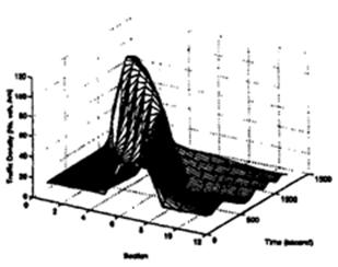
Fig. 2. Density profile without control.

 

In the second and third cases, we use the proposed controller to achieve desired traffic densities of 23 and 35 vehicles per kilometer respectively. The simulation results shown in Figs 4-9 demonstrate that the initial congested conditions are quickly dampened out by the proposed controller, and the traffic flow is regulated to achieve the desired traffic densities.

In the fourth case, we assume that the input traffic flow rate in section 1 increases exponentially from 1503 to 2000 vehicles per hour as shown in Fig. 10. We set the desired traffic density for this cast to 23 vehicles per kilometer. The simulation results shown in Fig. 11 show that the desired traffic density is achieved exponentially with the proposed road-way controller.

 

6. Conclusions

In this paper, we have considered the use of feedback for controlling traffic flow on the macroscopic level in an AHS environment. We have considered the design and analysis of such a roadway controller using a macroscopic traffic.

 

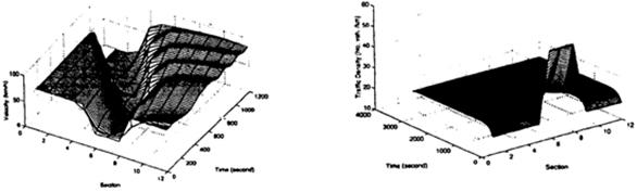
Fig. 3. Velocity profile without control.                                       Fig. 4. Density profile desired density

is 23 vehicles per kilometer.

 

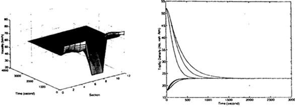
Fig. 5. Velocity profile desired density is 23                               Fig. 6. Density in each section desired

vehicles per kilometer.                                                     density is 23 vehicles per kilometer.

 

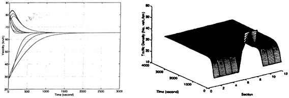
Fig. 7. Velocity in each section desired density                          Fig 8. Velocity profile desired density

is 23 vehicles per Kilometer.                                                           is 23 vehicles per kilometer.

 

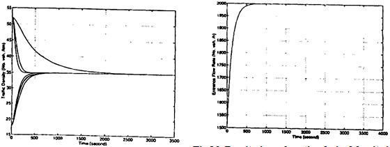
Fig. 9. Density profile desired density                          Fig. 10. Density in each section desired density

is 23 vehicles per kilometer.                                                            is 23 vehicles per kilometer.

 

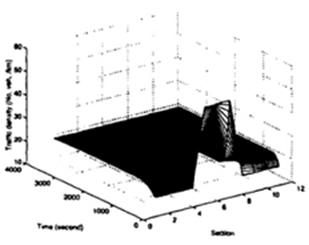
Fig. 11. Increasing entrance flow rate.

 

Flow model that is modified for AHS. The proposed controller has been shown to guar­antee exponential convergence of the traffic density to the desired one. Simulations have been used to demonstrate that an initial density disturbance can cause instability, which man­ifests itself as congestion in the absence of feedback control. The use of the proposed roadway controller demonstrates that such instability can be counteracted and congestion can be avoided.

 

References

 

1.                   Chien. C.C. and Iosnnou. P. (1992) Automatic vehicle following_ In Pox American Control Cont Chicago. IL. pp 1768-1752.

2.                   Chien. C. C. Iosnnou. P. and Chu. C. X. 11995) Fuzzy traffic density homogeneizer for automated highway sysleml Submitted to IEEE Fran,. Etta. Syr.

3.                   Creme.. M. and May. A. D. (1985) An encoded traffic model lac free.-ay control. Research Report 15CB^.ITS­RR-35 7.

4.                   Greenlee T L and Payne. H. J. (1977) Freeway ramp metering strategies for responding to incident+ In Pro (FEE conf on Decision and Control. pp. 982 .987 .

5.                   Hcdrkk, J.K., McMahon. D, Narendran, V_. end Swartoop, D (1991) Longitudinal vehicle controller design for 1VHS .pre system in proc American Cont. (Coot, Boston_, MA. pp. 3107-3112.

6.                   loannou, P and Chinn. C C. (1993) Autonomous Vnldligenl cruise control IEEE Tram Vrhfealar Trehnol 42, 657-672.

7.                   Ioennou, P.. Ahmcd^.7 id, F. and Wuh. D. 09971 A time headway autonomous intnlhgen cruise design and simulation Technical Report l,ISC^..SCT 9211.

8.                   K araselen, U. V.ratya, P and Walrand, J. (1990) Two propoula to improve freeway traf5c-1low Preprint.

9.                   Li1hlhill, M. J. and Whitham, G. B (1955) On kinematic waves ii: A theory of traffic flow on long crowded roads. Pros R Soc Lend. A229, 317-345.

10.               Papsgemgiou. M (1983) Apphcarionr of Automatic Control Conceper ro Traffic now Madding and ConrroL Springer-Vedag, Berlin.

11.               Pspegeorgiou. M. (1986) Freeway on ramp control strategies: overview, discussion and possible application to Boulenard Peipherique in Paris. Internal Report 1NRETS. Aroued, France.

12.               Papegeorgiou. M. Blosseville, 1. M. and Hadj-5alem, II. (1989) Macroscopic modeling of traffic flow on the Boulevard Periphorique in Paris. Traupon Re,. 13B, 29-47.

13.               Papageorge.. M, Blossevik. I. M. and Hadj-Salem, H. (1999a) Modeling and real time control on traffic flow on the southern part of Boulevard Periptrorique in Paris Part 1, Modeling. Transport Rel. 24A, 345-359.

14.               Papagcorgiou, M.. Blosaeville, J. M. and Haji-Salem. H. (1990b) Modeling and redaimc control of Traffic flow on the southern pan of Boulevard Peripherique in Paris. Pus II, Coordinated on-ramp metering. Transport Res. 24A. 361-370.

15.               Payne. H. J. (1971) Models of freeway traffic and cynitol. In Mathematical Models of Public Syarrnro. Simulation Council Proceeding, pp. 51-61.

16.               Payne, It, I. (1979) A Critical Preview of Microscope Freeway Model in Proc, Engineering Foundorlon Coif on Rnroreh Di.ecrrons in Computer Control of Urban Traffic 5y...no. pp. 251-265.

17.               Payne, H. 1.. Meisel. W. S and Teener, M D (1973). Ramp control to relive freeway congestion caused by traffic dislurhancealot. 1. Control 19, 52-64.

18.               Rao. P. S. Y., Vara.ye. P. and Eskan, F. (1992). Investiganons into achievable capecitks end strum stability .irh coordinated intelligent vehklea. PATH Technical Report.

19.               Sheikholeslam, S (1991) Control of a class of interconnected nonlinear dynamical system: the platoon problem Ph.D. dissociation. University of California, Berkeley.

20.               Shcikholeslam. S. and Desoer, C. A. (1991). A splcm level study of the longutidinal control of a platoon of "bides. ASME TDYn Syst., Meas , Control 114, 286-292.

21.               Shlodovcr, S. F.. (1991) Longitudinal Control of Automotive vehicles in Close-formation platoons. ASME I. Dya Sys.. Mono., Control 113, 231-241.

22.               Shladover, S E., Desoer. C A., Hedrick). K., Tomizoka, M Walrand, J. Z. Hang, W. B.. McMahon, D., Sheikholelslam. S.. Peng. H. and McKeown, N. (1991) Automatic vehicle control developments in the path pogrom. IEEE Trans. Vehicular Techno 114-130.

23.               Slotaky, A., Chico, C C and loannou, P. (1994) Robust platoon^. stable controller design (or autonomous intelligent "Vehicle. In Proc. 33rd IEEE Conf. on Decirion and Comm'. Lake Buena Vista, Fl„ pp. 2431-2436.

24.               Swaroop, D.. Chien, C. C., foannoo. P. and Hedrick, J. K. (1994). A comparison of sparing and headway control laws for Atomically Controlled vehicle. I. Vehicle 5pr. Dyer. 238.597-623.

25.               Yuanand, L 5. and Kreer, J. B. (1968) An optimal control Algorithm for romp metering of urban freeways In Proc. (6^th IEEE Annual Allerton Coot Circular and System Theory, University of Illinois, Allerton. IL.

 

Поступила в редакцию 21.09.2015 г.